As you know Excel has so many excellent features in it. Pivot Table is one of them. If you use Microsoft Excel and not used Pivot Table, It means you have missed a really great feature of Excel.

Pivot table is the best tool available in Excel to Sort, Filter, Count, Sum and summarizing the data in a worksheet. A pivot-table can automatically sort, count, total or give the average of the data stored in one table or spreadsheet. It displays the results in a second table, which is called as Pivot Table. Pivot table is also useful in preparing graph based on some calculated value from a data table.

This is very useful and easy to use. Despite of being so easy and useful, many people are scared of using Pivot Table. For them I must say, Do not scared of Pivot Table, start using them, soon you will become fan of Pivot table. So start using Pivot Table on every possible opportunities :).

As per Wikipedia “In data processing, a pivot table is a data summarization tool found in data visualization programs such as spreadsheets or business intelligence software”
 

Here in my Blog, I am writing a complete tutorial about Pivot Table. This is the first article of that Pivot Table Tutorial. In this article I am introducing Pivot Table to you. Remember, in future there will be so many articles coming as part of this tutorial. This one is just an Introductory article. So keep visiting this space to know more about Pivot Table.
 
If you want all the articles directly sent to your mailbox, Kindly subscribe yourself.

 

I am going to show How you can start using in Excel, by taking one simple Example.

Year	Product	Brand Name	Items Sold	Total Price
1990	Shoes	Nike	2300	4600000
1991	Shoes	Adidas	1800	3600000
1992	Shoes	Reebok	1200	2400000
1993	Shoes	Reebok	3200	6400000
1994	Shoes	Nike	1850	3700000
1990	Shoes	Reebok	500	1000000
1991	Floaters	Nike	700	1400000
1992	Floaters	Adidas	800	1600000
1993	Floaters	Reebok	200	400000
1991	Socks	Nike	2700	5400000
1992	Socks	Adidas	3800	7600000
1993	Socks	Reebok	4200	8400000
1991	Deo	Nike	13000	26000000
1992	Deo	Adidas	4500	9000000
1993	Deo	Reebok	3400	6800000
1995	Deo	Reebok	3600	7200000
1991	Perfume	Nike	13000	26000000
1992	Perfume	Adidas	4500	9000000
1993	Perfume	Reebok	3400	6800000
1999	Perfume	Reebok	3600	7200000

From the above table, You need to Find the below data using Pivot Table:
 
1. Total Items Sold for each Brand
2. Total Amount earned for each Brand

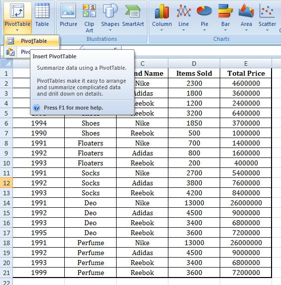
Step 1. Select the Table where Data is and Go to Insert –> Pivot Table

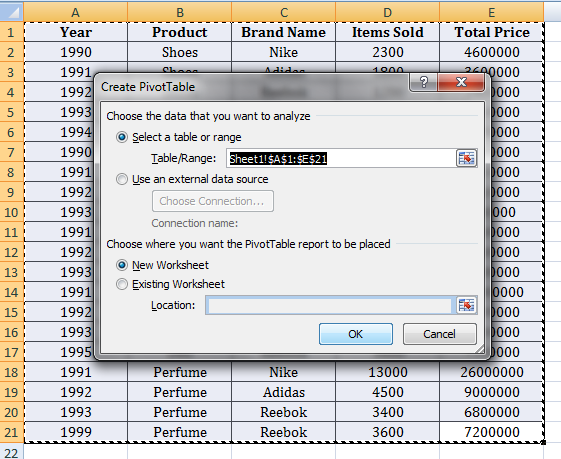
Step 2. Here you can see the selected Range with few options. Keep selected the default one.

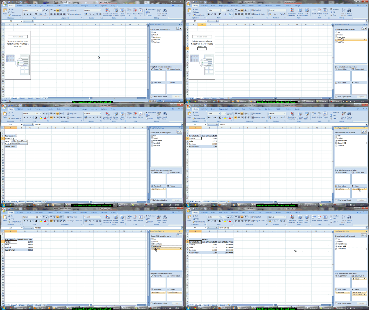
Step 3. A Pivot Table Place holder is inserted with the Options in Right hand side. Now refer the below moving Image, how to get the Sum of all Items sold and Price for each brand:

You can download this Excel from the below Download button, to practice Pivot Table. Keep looking this space to know more about Pivot Table.