Drop down list is made in Excel Cell to limit the Entry in to a Cell from a predefined set of values. It means you are restricted to select one value out of set of Predefined values. On creating a drop down list on a cell or cell-range, one drop-down will be displayed with set of predefined values, on selecting that cell and user can select one value out of that. You can not enter any value other than those predefined values.
Now we will see how to make Drop Down List in Excel 2003, 2007 and 2010.

• How to Create Drop Down in Excel 2003
• How to Create Drop Down in Excel 2007/2010
• How to Create Drop Down using named Range

How to Create Drop Down in Excel 2003

Follow below steps to Create Drop Down List in Excel 2003:

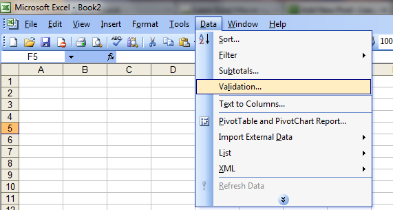
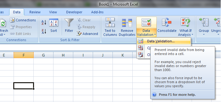
Step 1. Click on Data –> Data Validation option from the Top Menu

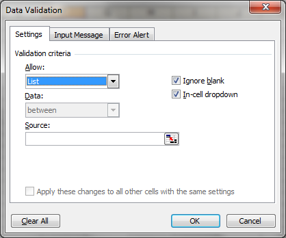
Step 2. In validation criteria Select “List” from the Drop down

Step 3. Click on Settings tab in the dialog box.

Step 4. Select “List”option from the Drop Down

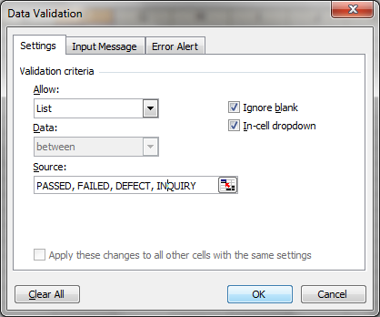
Step 5. Now Enter the List of Values in Source, you want to Add in the Drop down. Write all the Values separated by Comma (,).

Note: If you want to populate this list from the Values entered in to a Cell Range.

For Example: If you want to populate the Values from the Cell Range A1 to A5. So Enter the Source as =$A$1:$A$5. Whatever you enter in this Cell Range, will be shown in the Drop Down List.

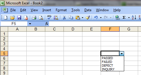
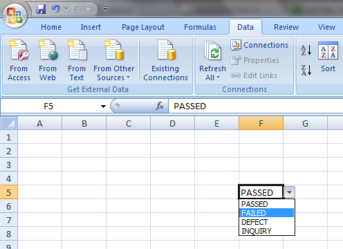
Step 6. A down arrow should appear in the Selected Cell as shown below.

How to Create Drop Down in Excel 2007/2010

Follow below steps to Create Drop Down List in Excel 2007/2010:

Step 1. Click on Data Tab –> Data Validation option from the Ribbon

Step 2. In validation criteria Select “List” from the Drop down

Step 3. Click on Settings tab in the dialog box.

Step 4. Select “List”option from the Drop Down

Step 5. Now Enter the List of Values in Source, you want to Add in the Drop down. Write all the Values separated by Comma (,).

Note: If you want to populate this list from the Values entered in to a Cell Range.

For Example: If you want to populate the Values from the Cell Range A1 to A5. So Enter the Source as =$A$1:$A$5. Whatever you enter in this Cell Range, will be shown in the Drop Down List.

Step 6. A down arrow should appear in the Selected Cell as shown below.

How to Create Drop Down using named Range

Follow below steps to Create Drop Down List using Named Range in Excel:

Step 1. For this first we need to make the Named Range in the workbook.
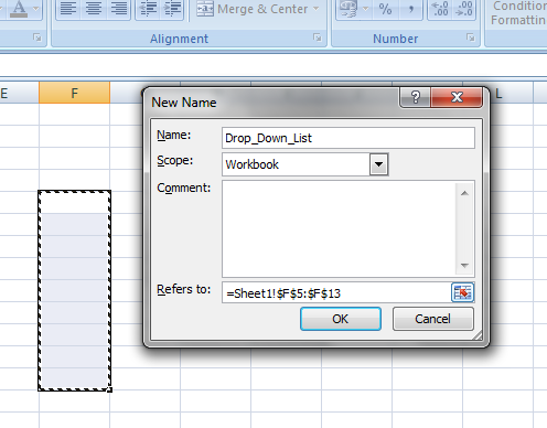
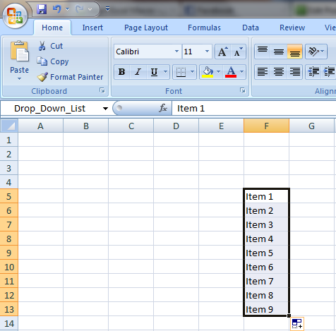
Step 2. To make the Named Range, Select the Range
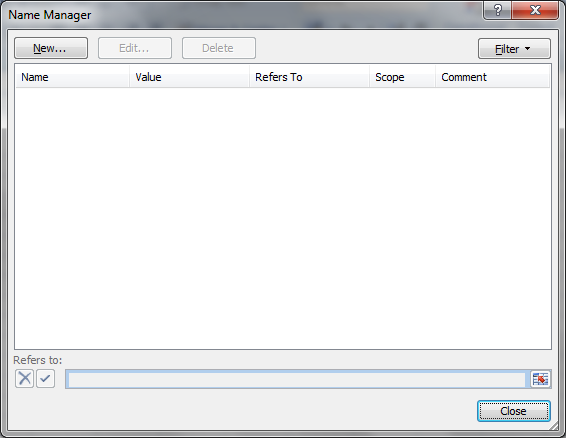
Step 3. Press Ctrl+F3



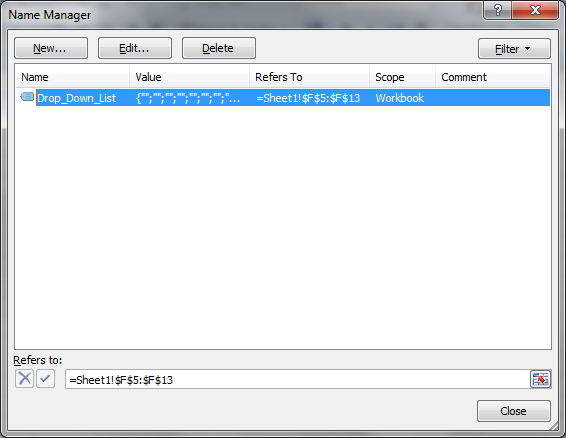
Step 4. Click on “New Button” in the Name Manager Dialog Box.



Step 5. Give a Name and Select the Scope
Step 6. Click OK



Step 7. Click Close.
Step 8. Now Ranged Name is created.



Step 9. To Create the Drop Down List Follow the below Instructions:
Step 10. Select the Cell or Cell Range where you want to Create the Drop down list.
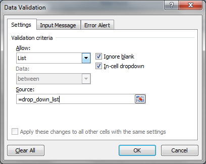
Step 11. Go to Data Validation –> Select List
Step 12. In Source Data enter =Ranged Name which is created above