The RANDARRAY() function is a powerful tool in Excel that allows you to generate arrays of random numbers. It is one of the dynamic array functions introduced in Excel 365, and it has quickly gained popularity due to its flexibility and versatility.
Note:
This is the last article of Dynamic Arrays and Spill Functions in Excel series. In this series we are going to learn about FILTER(), SORT(), UNIQUE(), SEQUENCE() functions.
Syntax:
RANDARRAY({rows}, {columns}, [min], [max], [integer])
Where:
- Rows (Optional): This number dictates how many rows your array will occupy. Feeling generous? Fill a hundred rows with a single formula! Minimum: 1.
- Columns (Optional): Spread your randomness across columns! Define the desired column width for your array. Minimum: 1.
- Min (Optional): Set the lower limit for your random numbers. Default: 0.
- Max (Optional): Define the upper limit for your numerical playground. Default: 1.
- integer (Optional): True for integers, False for decimals (default). Unleash the power of whole numbers or embrace the beauty of decimals!
Notes [Use cases]:
- Unlike its static cousin RAND(), RANDARRAY() updates automatically whenever you change the worksheet, keeping your data fresh and ever-random.
- Nest RANDARRAY() within other functions like IF or SUM to create custom random number distributions. Get creative!
- Generate random lottery numbers within a specific range using RANDARRAY(). Remember, winning is still up to chance!
With its flexibility and dynamic nature, RANDARRAY() is a powerful tool for data generation and exploration in Excel. So, next time you need a dose of randomness, ditch the manual methods and harness the power of this dynamic function. Remember, with great randomness comes great responsibility…use it wisely, and have fun!
Generate array of random numbers in Excel
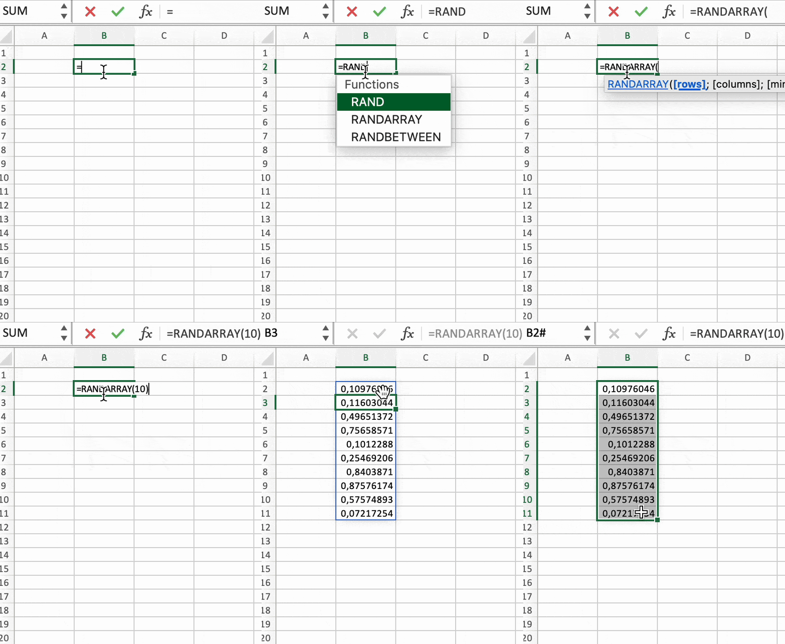
Lets say you want to generate 10 random numbers from row1 i.e. the row where your formula is typed, till the 10th row, you can simply pass the only row parameter in the formula as shown in the below picture.
=RANDARRAY(10)
Random Number Array – Rowsie
The above random numbers generated are spread across 10 rows because the first argument passed in the formula is the count of rows where you want to spread the random numbers. Rest other parameters are used as default one. By default, it generated random numbers in the same column where formula is typed. The default min and max is between 0 and 1 — therefore you can see all the random numbers generated are less than 1. Default value of last optional parameter i.e. integer is set to false. That means, by default it generates decimal numbers as random numbers.
Random integers between a custom range in Excel
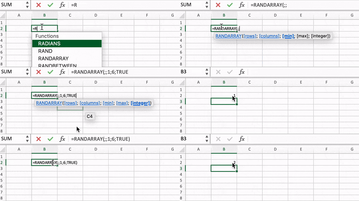
Let’s imagine you want to create a game where you want to roll a dice. Every time a dice is rolled only an integer between 1 and 6 should appear. In this case, you can provide min and max parameter as min=1 and max=6 and set the integer boolean to true. This way it will always generate a random number between 1 and 6. No decimal value.
=RANDARRAY(,,1,6,True)
Random Integer Array in Excel
Everytime, formula is refreshed a new random integer between 1 and 6 is generated. Ensure min is less than max, otherwise you’ll get an error. Ensure max is greater than min, otherwise you’ll get an error.
Matrix of Random Integers in Excel
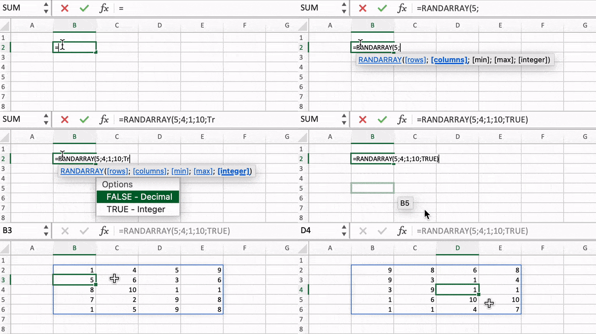
Let’s imagine you want to create a matrix of size 5X4 of random integers between 1 and 10, you can simply use following formula by providing all the parameters of RANDARRAY function in excel.
=RANDARRAY(5,4,1,10,True)
Random Array Integer matrix – Excel
Remember:
- All parameters are optional, and omitting them uses default values (rows=1, columns=1, min=0, max=1, whole_number=FALSE).
- Combine these parameters to create arrays of random numbers tailored to your specific needs.
- Use RANDARRAY() responsibly and have fun exploring the world of randomness in Excel!




0 Comments