This is the 4th article of Dynamic Arrays and Spill Functions in Excel series. In previous articles, we have learned about FILTER(), SORT(), UNIQUE() and RANDARRAY() functions of this series.
In this article, we will learn about yet another Dynamic Array function called SEQUENCE(). This function was introduced in Excel 365 and Excel 2019. In this article, we will dive into the details of the SEQUENCE() function, exploring its syntax, various use cases, and tips to maximize its potential.

Understanding the Syntax:

The SEQUENCE() function has a straightforward syntax:

SEQUENCE(rows, [columns], [start], [step])

Where:

1. rows: The number of rows in the sequence.
2. [columns] (optional): The number of columns in the sequence. If omitted, it defaults to 1.
3. [start] (optional): The starting value of the sequence. If omitted, it defaults to 1.
4. [step] (optional): The increment between values in the sequence. If omitted, it defaults to 1.

The beauty of the SEQUENCE() function lies in its dynamic nature. When used as the final result of a formula, the array it generates will automatically expand to fill any empty cells below and to the right of the formula. This flexibility allows you to create arrays of varying sizes without manual resizing. Now, lets understand them by using few examples.

Basic Example of using SEQUENCE()

If you want to generate a number series from 1 to 5 in a column from Row 2 to Row 7, you can simply type the following formula in Row 2 of that column as shown in the picture below:

SEQUENCE(5)

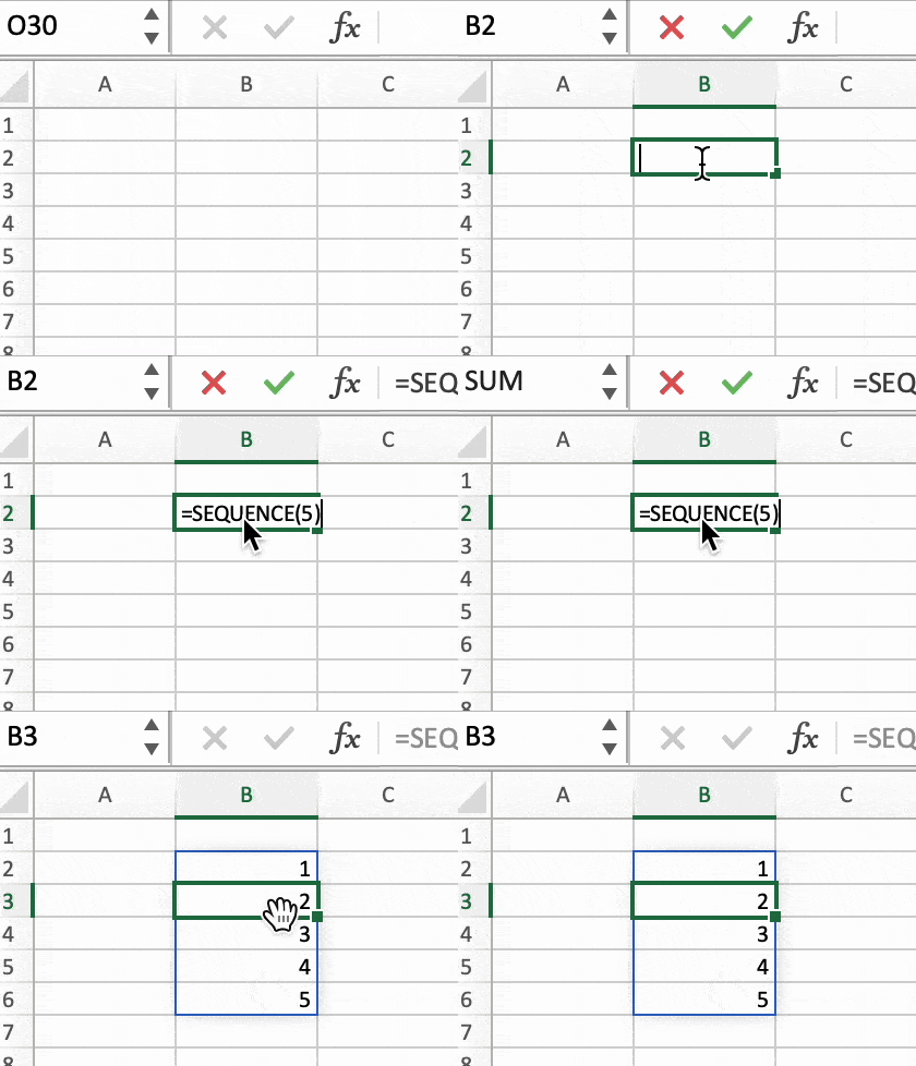
SEQUENCE() Formula

Specifying Rows and Columns in SEQUENCE() Funciton

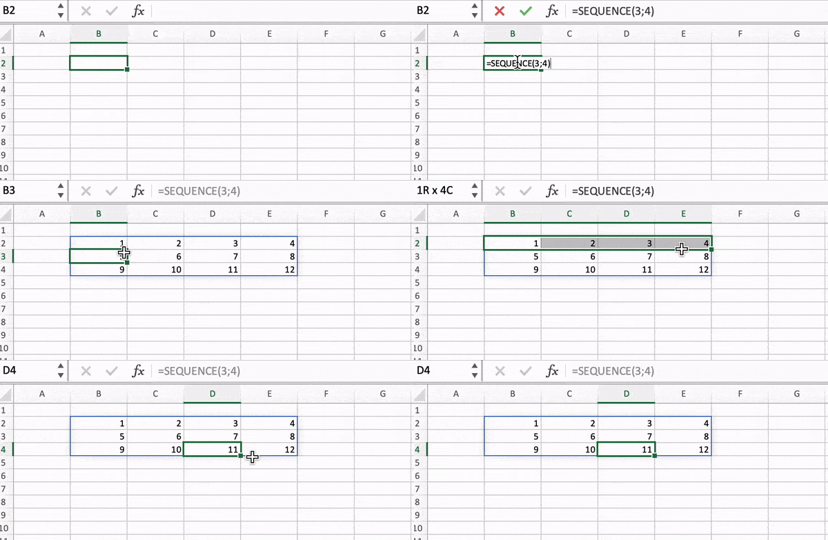
In the above example, you had provided the number of rows only. That is the only mandatory parameter for this function. Here in this case, you can provide both rows and columns and see how it works.

SEQUENCE(3, 4)

Sequence-function

Here, a 3×4 matrix is created with sequential numbers. The sequential numbers are written column-wise.

In the above examples as you can see all the numbers are written in sequence difference by 1. Example : 1,2,3,4…

SEQUENCE() function with Custom Start and Step Values:

What if you want to generate a sequence with a specific difference between two numbers. For example, you want to generate a sequence starting from 5, 10, 15, 20, … etc. In this case, we can simply set the Start parameter to 5 and Step parameter to 5.

SEQUENCE(4,,5,5)

In the above example, I have skipped the column parameter but passed the start and step parameters as 5. Therefore, above function will generated 4 numbers starting from 5, 10, 15 and 20. You can refer in the below picture.

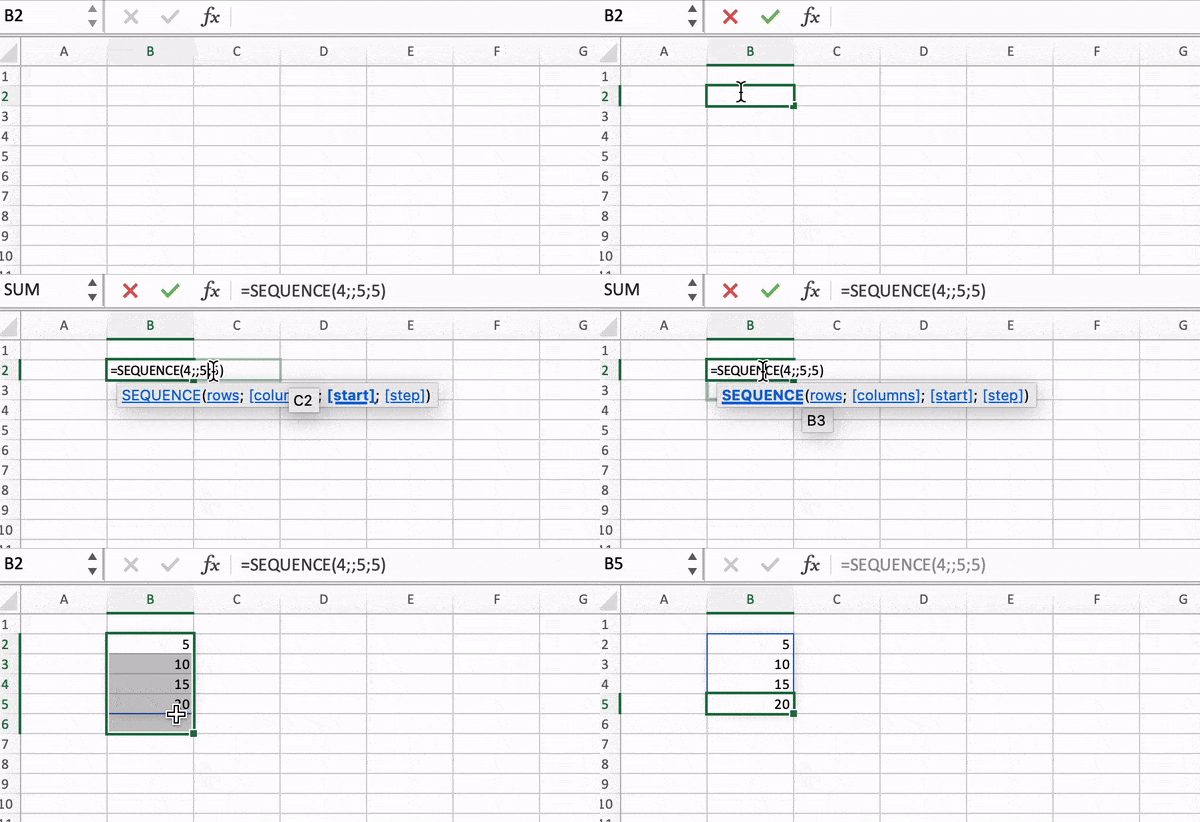
Custom Start and Step in Sequence()

Tips and Tricks

Here are some additional tips and tricks for using the SEQUENCE() function effectively:

1. Always use enough empty cells below and to the right of the formula when using the SEQUENCE() function as the final result.
2. If you’re using the SEQUENCE() function within another formula, ensure that the final result is enclosed in curly braces ({ }) to create a dynamic array.
3. The SEQUENCE() function works well with other dynamic array functions like SUMPRODUCT and INDEX/MATCH.