In today’s tutorial, we’ll be diving into the exciting world of dynamic arrays and spill functions in Excel. These features have revolutionized the way we work with data, providing a more flexible and efficient way to handle arrays. I am going to explain these concepts step by step with examples that are perfect for all beginners till expert.
Note:
This is the 2nd article of Dynamic Arrays and Spill Functions in Excel series. In this series we are going to learn about FILTER(), SORT(), UNIQUE(), SEQUENCE() and RANDARRAY() functions.
The next function we are going to learn is the SORT() function.
It allows you to sort specific data from a range based on the provided order and returns, an array of sorted values
Here "returning an array" is noteworthy in this formula. Unlike most of the excel formula, this does not return a single value rather it returns a series of values. This makes this excel formula special.
FREE! Playground and Download
Do not forget to play around the embedded excel sheet at the end of this article.
Syntax of Sort() formula
Following is the syntax of Sort formula
=SORT(array, [sort_index], [sort_order], [by_col])
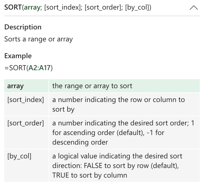
Sort Formula
Explanation about the parameters
array:The range or array you want to sort.sort_index: (Optional)The column or row number in the array to sort by. If omitted, the entire array is sorted.sort_order: (Optional)The order of sorting: 1 for ascending, -1 for descending. If omitted, it defaults to ascending order.by_col: (Optional)TRUE to sort by columns, FALSE to sort by rows. If omitted, it defaults to FALSE.
Example: Sorting the Sales Data
Let’s say you have a list of sales data as shown in picture below. You want to sort the products with sales amount. So one option is to use the excel’s built-in sorting feature available on a table and sort the rows by sales amount column according to your wish. But note that, this option will simply rearrange your same source table data. It will not create a copy of sorted data. If you want to have your sorted data in some other cell then, Sort() formula will help you.
Input Data:
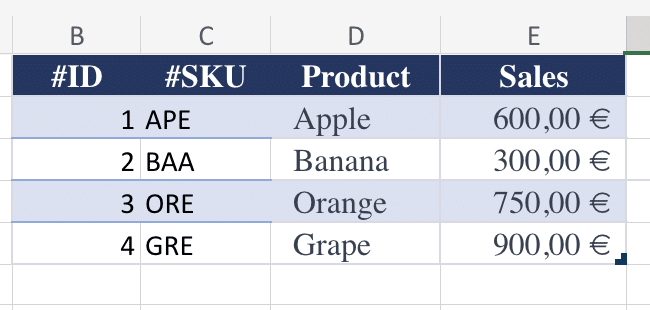
Sales Data Table – Filter Formula
=SORT(B2:E5;4;1;FALSE)
Explanation:
B2:E5-This is the range of data you want to sort4– From the above range, this is the column number [index number] which you want to sort it. For example, in this case, Sale amount is4thcolumn in B2:E5 range1-The order of sorting:1for ascending and-1for descending.FALSE-False means you want to sort the data – row-wise. If you want to sort the data column-wise, you can set it toTRUE
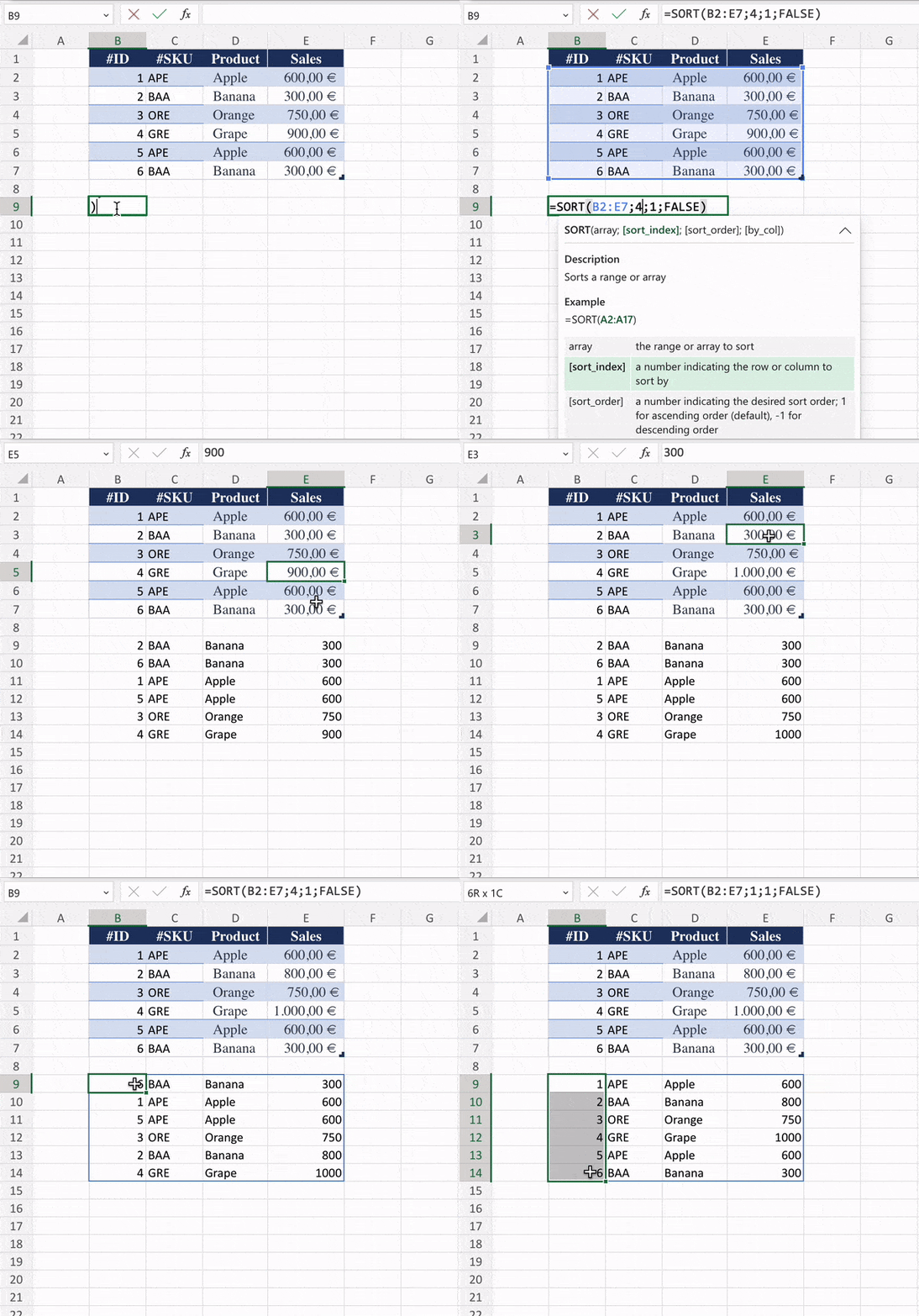
Sort Function in Excel
Sorting by Multiple Columns using SORT() Formula
To sort by multiple columns, you can use the array argument to specify the columns you want to consider. For example, to sort by the first column in ascending order and then by the second column in descending order, you can use:
=SORT(A1:C10, {1,2}, {1,-1}, FALSE)
-
Dynamic Spill Range:The SORT() function automatically spills results into adjacent cells, creating a dynamic spill range. Column-wise sortingUsing SORT() formula, it is possible to sort the data column-wise too.Sorting by Multiple ColumnsUsing SORT() formula, it is possible to sort the data by multiple columns, each in different order as shown in the above example.
Conclusion:
Congratulations! You’ve successfully explored the SORT() function in Excel. This versatile tool empowers you to sort the data precisely the way you want. Stay tuned for more Excel insights and tutorials!
Your Playground: Excel Workbook
Now in the below excel workbook, you can play around with the SORT() formula by providing different types of parameters.




0 Comments