In today’s tutorial, we’ll be diving into the exciting world of dynamic arrays and spill functions in Excel. These features have revolutionized the way we work with data, providing a more flexible and efficient way to handle arrays. I am going to explain these concepts step by step with examples that are perfect for all beginners till expert.
Note:
This is the first article of Dynamic Arrays and Spill Functions in Excel series. In this series we are going to learn about FILTER(), SORT(), UNIQUE(), SEQUENCE() and RANDARRAY() functions.
The first such function we are going to learn is the FILTER() function.
It allows you to extract specific data from a range based on given criteria, returning an array of values that meet the specified conditions.
Here "returning an array" is noteworthy in this formula. Unlike most of the excel formula, this does not return a single value rather it returns a series of values. This makes this excel formula special.
FREE! Playground and Download
Do not forget to play around the embedded excel sheet at the end of this article.
Syntax of Filter() formula
Following is the syntax of filter formula
=FILTER(array, include, [if_empty])
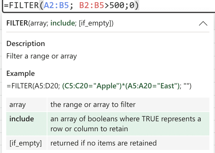
Filter Formula
Explanation about the parameters
- array (mandatory): The range of data you want to filter.
- include (mandatory): The conditions that the data must meet to be included in the filtered result.
- [if_empty] (optional): What to return if no data meets the specified conditions.
Example: Filtering Sales Data
Let’s say you have a list of sales data as shown in picture below. You want to filter out the products with sales greater than 500. So one option is to use the excel’s built-in filter feature available on a table and filter only those products that have sales higher than 500. But note that, this option simply hide those rows which does not meet the criteria. It does not create a separate sub-set of your original table by filtering those records which are meeting the criteria provided by you.
If you want to create a separate sub-set of your original data by applying some filter conditions, you can use Filter() formula in excel.
Input Data:
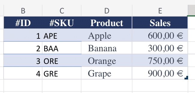
Sales Data Table – Filter Formula
=FILTER(B2:E5, E2:E5>500, "No Products Found")
Explanation:
array (B2:E5):This is the range of data we want to return for which conditions are met. In this case, it should return values from two columns B to E.include (E2:E5>500):This condition specifies that only sales greater than 500 should be included in the result.[if_empty] ("No Products Found"):If there are no sales exceeding 500, the function will return “No Products Found”
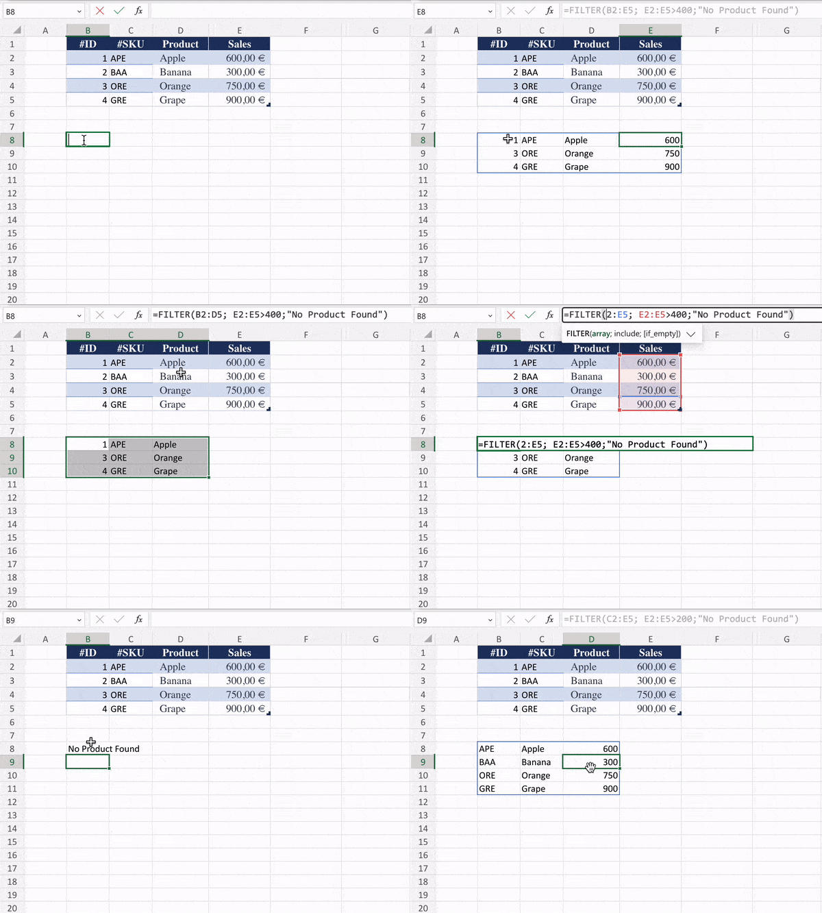
Filter Function in Excel
-
Dynamic Spill Range:The FILTER() function automatically spills results into adjacent cells, creating a dynamic spill range. Multiple Conditions:You can use logical operators (AND, OR) to apply multiple conditions within the “include” parameter.Tips and Best Practices:Named Ranges: Consider using named ranges for your array parameter to enhance formula readability.
Conclusion:
Congratulations! You’ve successfully explored the FILTER() function in Excel. This versatile tool empowers you to extract precisely the data you need based on specified conditions. Experiment with different scenarios, and remember the flexibility and power this function brings to your data analysis toolkit. Stay tuned for more Excel insights and tutorials!
Your Playground: Excel Workbook
Now in the below excel workbook, you can play around with the Filter() formula by providing different kind of filter criteria, range etc.
Try adding multiple criteria and filter.




0 Comments
Trackbacks/Pingbacks