Dear Readers,

In this article I am going to explain you, how you can format the Alternate Rows of Excel using Conditional Formatting. For example, in Excel Sheet, if you want alternate rows to be shaded in different color. This you usually need when you are preparing some report and want your report looking very nice.
Follow the below Steps to do so:

Steps to Shade Alternate Rows (Automatically)

Step 1.Select the Area which you want to be shaded. If you want the whole Sheet to be formatted then Select the whole sheet.
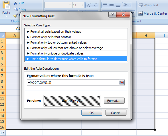
Step 2. Go to the Home Tab in the Menu Ribbon (Excel 2007) –> Click on Conditional Formatting Option
Ste 3. Click on Add New Rule
Ste 4. Select the Format Type as “Use a Formula to Determine Which cells to format”

Shading Alternate Rows

Ste 5. Type this formula =MOD(ROW(),2)
Ste 6. Click on Format Button and change the format, how you want.
Ste 7. Click OK
Ste 8. Click OK

Shading Alternate Rows

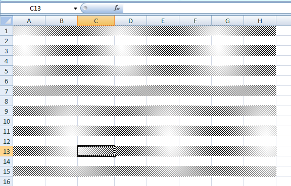
Now you can see that in your Selected Area, all the Alternate Rows will be having the same Formatting what you had chosen in the above dialog.

Brief Explanation:

In the above formula I have used MOD and ROW() function. ROW() Function returns the Row Number like 1, 2, 3, 4 etc.
Now the MOD() Function will return Alternatively: 1, 0, 1, 0.
And because of that Alternatively the Shade of the row will be formatted as shown above picture.

How is it different than Simple Formatting by Selecting the Alternate Rows?

1. In simple formatting if you want to delete any row in between then the whole formatting will messed-up and you need to format it again till end (alternatively) but using conditional formatting as soon as you delete any row rest all will be automatically formatted alternatively.
2. Get rid of alternate selection and then filling color and all in it to look good… give this task to conditional formatting.. it will do 🙂 You just enjoy the formatting done automatically.