Sometimes in Excel, we need auto-formatting as soon as a condition in a particular cell or cell range is satisfied then the formatting of the whole row or a cell range should change. This is very easy to do in Excel by using Conditional Formatting.
Let’s take an example. Suppose you have the following data in the Excel Sheet

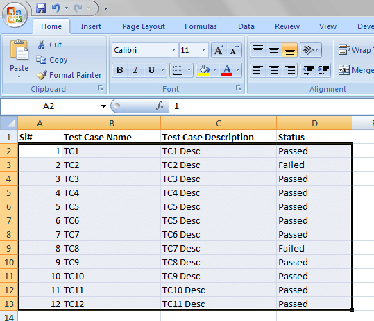
Conditional Formatting for Range

In the above format, you want that as soon as you select Status as “Failed” then for that row, all the Columns like Column A, Column B, Column C, and Column D, color should change to Red.

Now Select the Whole Range, where you want to Apply the formatting as shown in the above Picture.

Go to Home Tab –> Conditional Formatting
Now Click on Use a formula to determine which cells to format
In the formula bar, Enter the formula: =$D2=”Failed” as shown in the Picture.
Note: In the formula make sure that you are using $ Sign before the Column Name. But you should not use this sign before Row Number.

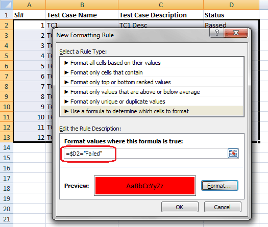
Conditional Format on Range

Click OK
Now you can see that the selected Row color is changed to Red where ever Status is Selected as “Failed”. Refer below screen-shot.

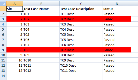
Conditional Formating on Range

Now if you want to change the Color of that complete row wherever the Status is Failed then Follow the below Steps:

Step 1.While Selecting to format, Select the Complete row and then Apply the Conditional Format.

OR

Step 2. Edit the Existing Conditional Formatting by Clicking on Manage Rules in Excel 2007.
In Manage Rules, Enter this Range in Applies To Field.
When you want to format complete row to be formatted then in “Applies to” Field DO NOT enter Column Names.Just you need to Enter the Row Range. Like $1:$1200 as shown below.

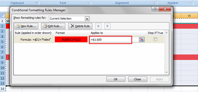
Conditional Formatting On Range