Conditional Formatting in Excel:

In MS Excel we can do formatting of cells based on some conditions or values. This is called Conditional formatting. For example, if you want a cell color to be red whenever the Value in the Cell is updated as “FAILED” or “Less Than 60%” etc. then we can apply conditional formatting in that cell.
Conditional formatting can be done on a single cell or a range of cells or in complete row or column.

Excel 2007:

Following are the steps to do Conditional Formatting in Excel 2007:

Step 1. First of All Select the Cell or Cell Range where you want to apply this conditional formatting

Step 2. Go to Home Tab –> Conditional Formatting –> New Rule

Conditional-Formatting

Step 3. Here there are many types of conditions like you want to do formatting based on any custom formula, or on a cell value etc. Select the option whichever is suitable for you and enter the conditions accordingly

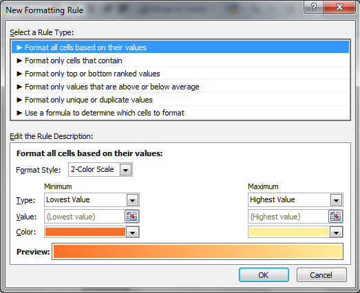
Step 4. For example i am selecting “Format only cells that contains”

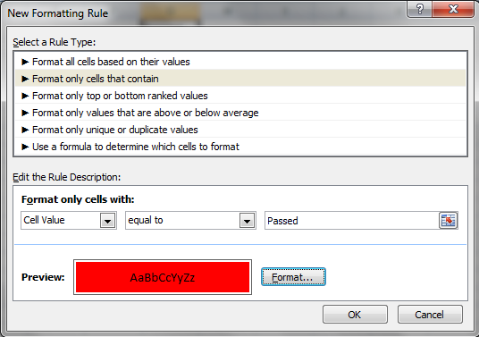
Step 5. Now select the Condition as ** Cell Value ->Equal to ->”Passed” **.

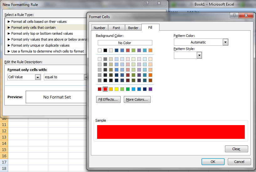
Step 6. Select the Formatting of the Cell by clicking on the Format Button in the below dialog box.

Step 7. Click ok

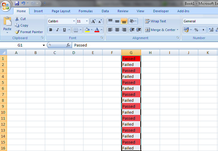
Step 8. Now All the cells which are having value as “Passed”, formatting automatically got changed as per the selected condition.

Note:Now as soon as we change the Value of a cell as “Passed” in the selected range then the Color of the cell will be automatically changed to “Red”

Excel 2003:

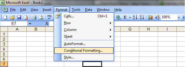
Following are the steps to do the Conditional Formatting in Excel 2003:

Step 1. Select the Cell or Cell Range where you want to apply the conditional formatting.
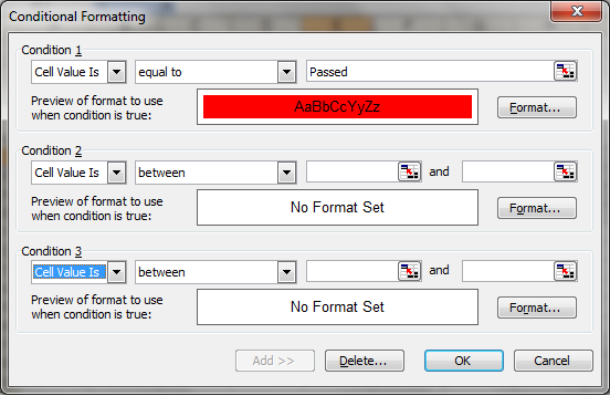
Step 2. Go to Format –> Conditional Formatting

Step 2. Now Select your Condition and Formatting accordingly

Step 3. Click ok

And here your conditional formatting is done.

Read this Also:

• Edit Conditional Formatting
• Conditional Formatting based on condition in other cell