In previous post we saw the normal conditional Formatting. It means based on the condition of a cell, changing the format of same cell is normal conditional formatting. But here we are going to see the conditional formatting of a cell based on some other cell condition. Suppose if you want to change the formatting of a cell based on condition on some other cell then follow the below steps:
Example: I want to change the Color of cell A1 if the Value of cell E1 is less than 5

Step 1. Select the Cell A1
Step 2. Go to Home –> Conditional Formatting –>New Rule

Conditional Formatting

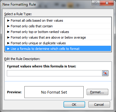
Step 3. Select “Use a formula to Determine which cell to Format”

Step 4. Enter the Formula in the Formula Bar in the below Dialog
DO NOT put $ sign in the Cell Name for the Formula. If you are putting $ sign in the Cell Name like “$E$1” then this Conditional formatting will be applied only on this cell. If you want this formatting to apply on whole column then your formula should be like this “=E1<5"

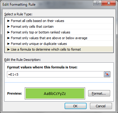
Conditional formatting

Step 5. Click ok
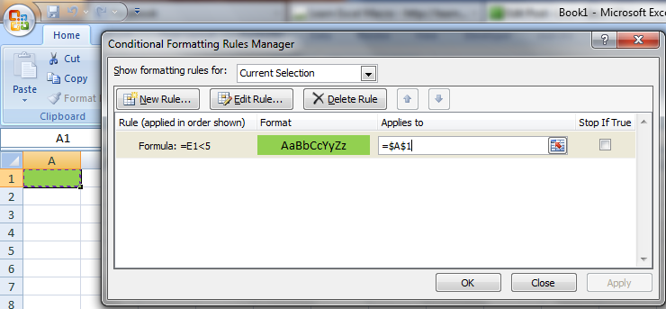
Step 6. Go to Home –> Conditional Formatting –>Manage Rules
Step 7. Now here you can change the Cell range in the “Apply To” field (as shown below) where you want to apply this conditional formatting.

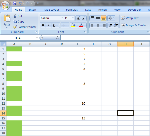
Step 8. After applying this Formatting on whole column, formatting of Column A will be done automatically as soon as we change the value in E column as shown below:

Read this Also:

• Conditional Formatting
• How to Edit Conditional Formatting